PyMC3 tutorial on Mixture Models
3/6/2021 • PA,USA
In this post, I talk about using PyMC3 to create a probabilistic model to estimate parameters of a mixture model using simulated data. I have used a mixture modeling approach in the past to predict the accuracy of planar, laser-based experimental imaging for measuring flame speeds in turbulent flames. You can read more about it in this paper.
For this post, I am creating synthetic data mimicking a sphere shrinking in size and moving in space, while passing through a fixed plane. From the context of my PhD work, the sphere represents a pocket of unburnt fuel+air mixture surrounded by a reaction zone (the flame, where combustion occurs), the shrinking process represents the consumption of those gases, and the fixed plane represents the plane of laser-based imaging. The motion of this sphere represents the convective motion of the flame pocket. The rate of shrinking represents the consumption speed of unburnt gases surrounded by the flame or ‘flame speed’. If 3D measurements are made, this rate would be represented as follows:
$$S_{C,3D} = \frac {\Delta V} {S_{a} \Delta t} $$
where, \(\Delta V\) is the volume change in \(\Delta t\) over volumetric surface area \(S_{a}\). 3D measurements are quite complex to perform and many researchers rely on 2D measurements, so the 2D version of this equation would be:
$$S_{C,2D} = \frac {\Delta A} {P \Delta t} $$
Here, \(\Delta A\) is the change in 2D area in time \(\Delta t\) over the perimeter \(P\). With 2D measurement, however, there is an uncertainty with the three-dimensionality of the flame and how it impacts the interpretation of the 2D measurements.
First, I create synthetic data by statistically modeling the following four processes independently:
• Shrinking or consumption of the sphere: \(S_{C,3D} = S_{C,3D0} (1+\gamma)^{t/\Delta t}\)
• Initial size of the sphere: \(r_{0}\)
• Location of the fixed plane with respect to the sphere: \(z_{0}\)
• Bulk convective motion of the sphere: \(U_{z,0}\)
This modeling approach assumes that these processes are independent and can be randomly sampled as follows:
$$S_{C,3D0} \thicksim \Gamma(\alpha,\beta)$$ $$r_{0} \thicksim \mathcal{U}(r_{1},r_{2})$$ $$z_{0} \thicksim \mathcal{U}(0,z_{max})$$ $$U_{z,0} \thicksim \mathcal{N}(\alpha,\beta)$$
from matplotlib import pyplot as plt
import numpy as np
import pymc3 as pm
import pandas as pd
import seaborn as sns
import theano.tensor as tt
import math

SEED = 383561
np.random.seed(SEED)
# Modeling the initial consumption/shriking value of the sphere,
# the initial radius of the sphere, the initial location of the fixed plane,
# and the bulk convective motion of the sphere
with pm.Model() as model:
    Sc3D0_s = pm.Gamma('Sc3D0_s', 3, 1)
    r0_s = pm.Uniform('r0_s', 1e-3, 5e-2)
    z0_s = pm.Uniform('z0_s', 0, 2)
    U0_s = pm.Normal('U0_s', 0, 1)

# Run the PyMC3 model. Here, the burn-in sample size is 1000.
with model:
    trace = pm.sample(5000, n_init=10000, tune=1000, random_seed=SEED)[1000:]
Auto-assigning NUTS sampler...
Initializing NUTS using jitter+adapt_diag...
Multiprocess sampling (2 chains in 2 jobs)
NUTS: [U0_s, z0_s, r0_s, Sc3D0_s]
Sampling 2 chains, 0 divergences: 100%|██████████████████████████████████████| 12000/12000 [00:17<00:00, 702.43draws/s]
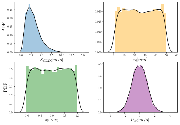
Using the samples generated above, I first generate synthetic 3D consumption rates using the equation \(S_{C,3D} = S_{C,3D0} (1+\gamma)^{t/\Delta t}\). Then, using the randomly distributed fixed planes, I calculate what the 2D consumption rates are in those planes when the sphere is moving and not shrinking (frozen in size).
g_rate = 0.01
it = 200
delt = 0.001
t = np.zeros(it)

Sc3D_data = []
Sc3D_data2 = []
Sc2D_data = []

for kk in range(100):
    Sc3D = np.zeros(it)
    Sc3D[0] = Sc3D0_s[kk]

    r = np.zeros(it)
    r[0] = r0_s[kk]

    z = np.zeros(it)
    z[0] = r0_s[kk] * z0_s[kk]

    Uz = U0_s[kk]

    r2D = np.nan * np.zeros(it)
    r2D[0] = (r[0]**2 - (r[0] - z[0])**2)**0.5

    Sc2D = np.nan * np.zeros(it)

    # Loop to create exponentially growing consumption rates and...
    # to find the radius as a function of time based on those consumption rates
    for ii in range(it-1):
        t[ii+1] = t[ii] + delt
        Sc3D[ii+1] = Sc3D0_s[kk] * (1 + g_rate)**ii
        Sc3D_data.append(Sc3D0_s[kk] * (1 + g_rate)**ii)
        r[ii+1] = (r[ii]**3 - ((Sc3D0_s[kk] * (1 + g_rate)**ii) * delt * r[ii]**2))**(0.3333)
        z[ii+1] = z[ii] - (Uz*delt)
        if (r[ii+1]**2 - (r[ii+1] - z[ii+1])**2) >= 0:
            r2D[ii+1] = (r[ii+1]**2 - (r[ii+1] - z[ii+1])**2)**0.5
            Sc2D_data.append((r2D[ii]**2 - r2D[ii+1]**2)/(2*r2D[ii]*delt))
            Sc3D_data2.append((r[ii]**3 - r[ii+1]**3)/(3*(r[ii]**2)*delt))
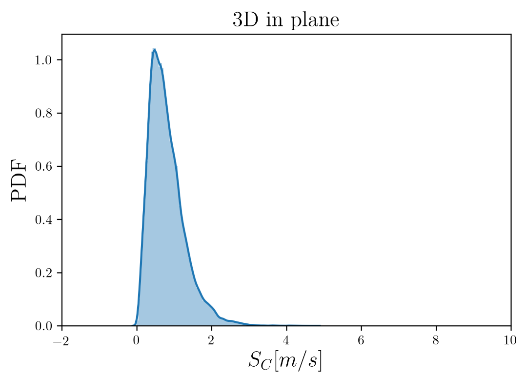
Distributions of the 3D and 2D consumption rates of the spheres in randomly distributed planes are shown below. If we look at the distribution of the 2D measurements, we see that there are some negative values. We can anticipate that these negative points (and some of the positive values) can be attributed to the motion of the 3D sphere being in a fixed plane rather than the actual shrinking/consumption of the sphere.
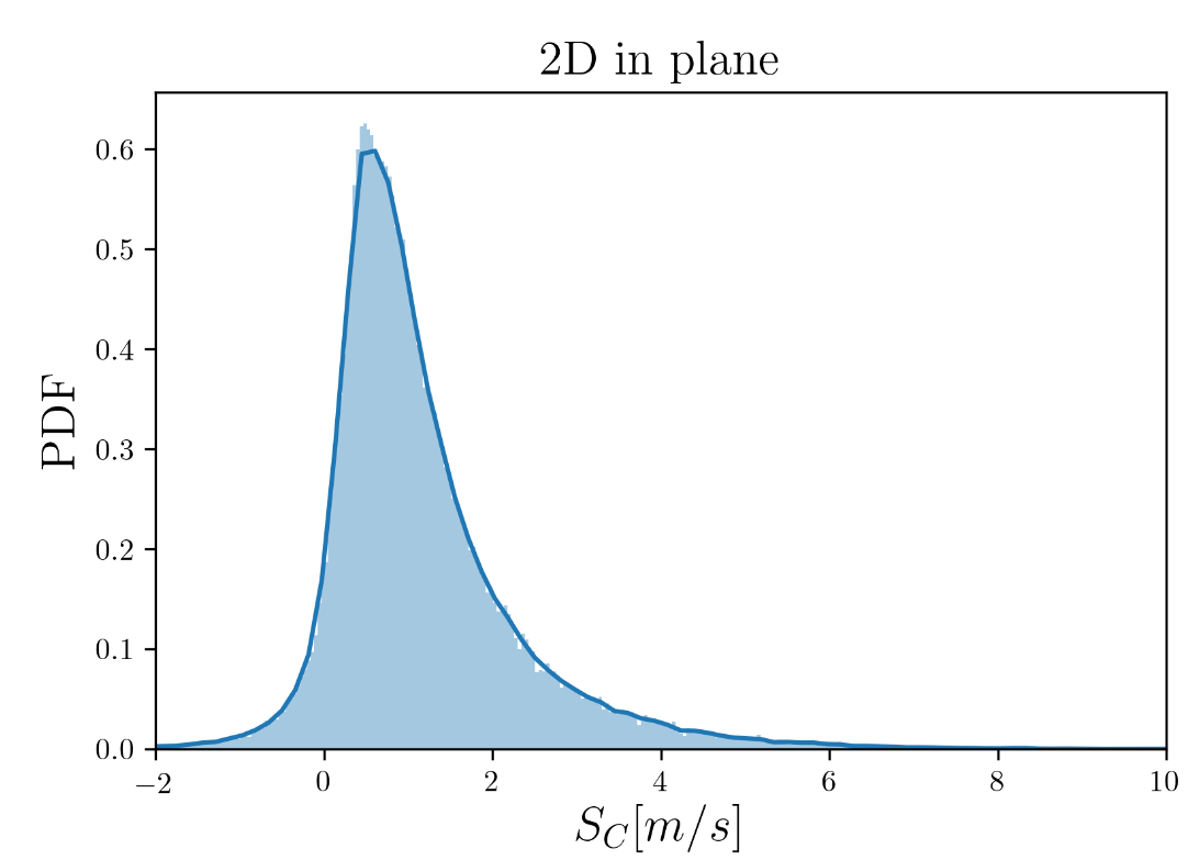
Distribution of the 2D consumption rates of the frozen spheres in the same randomly distributed planes are shown below. This distribution is pseudo-symmetrically distributed about zero.
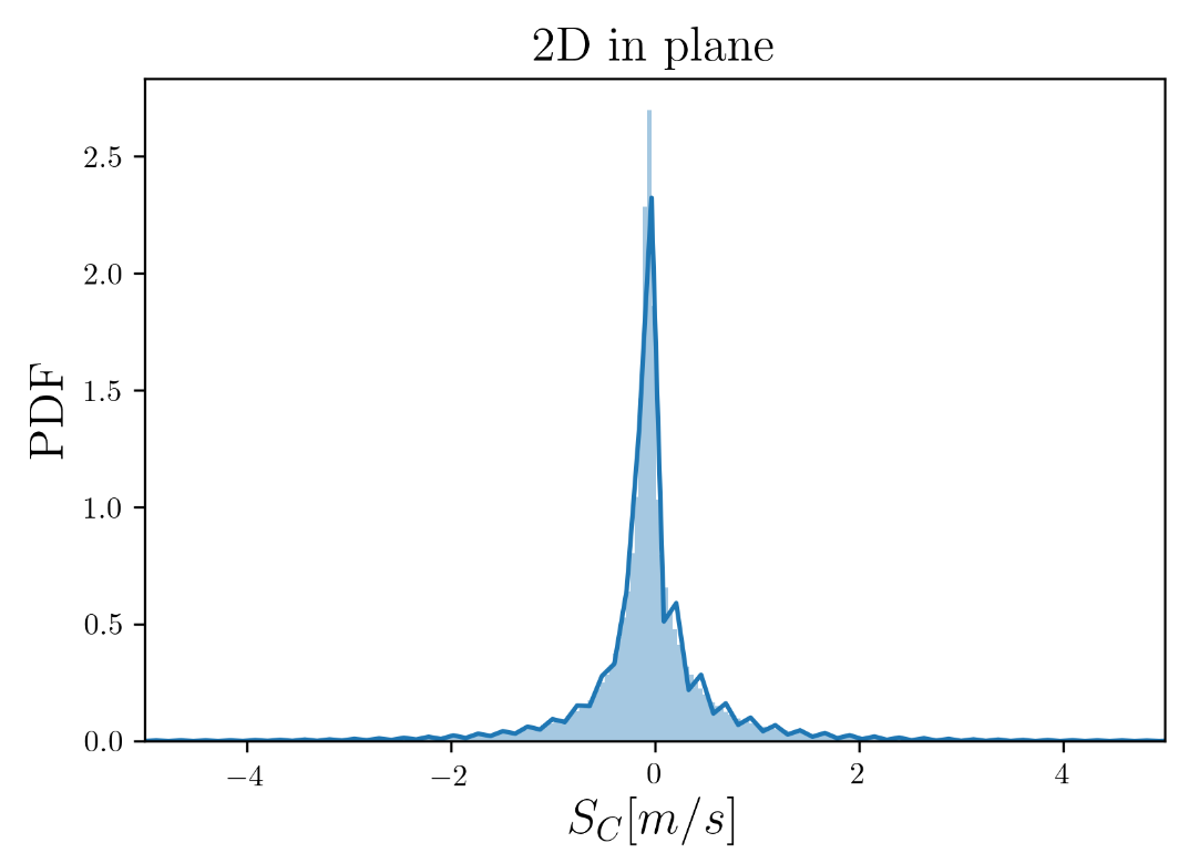
In order to isolate the effect of the 3D motion, I use a mixture model approach to statistically deconvolute this effect from the consumption rates in 2D. The 3D consumption rate distribution resembles an Inverse-Gaussian distribution and the ‘frozen’ 2D consumption rate distribution looks more like a Cauchy distribution.
Since we can know the parameters of the Cauchy distribution (\(f_{1}\)), we can fix those parameters in the mixture model.
$$f_{1} (x | \mu_{1},b_{1}) = \frac{1}{\pi b_{1}} \bigg( \frac{b_{1}^{2}}{(x-\mu_{1})^{2}+b_{1}^{2}} \bigg) $$
Then, we can use MCMC sampling methods to estimate the parameters of the Inverse-Gaussian distribution (\(f_{2}\)).
$$\mu_{2} \thicksim \Gamma(\alpha=1,\beta=1)$$ $$\lambda_{2} \thicksim \Gamma(\alpha=1,\beta=1)$$
$$f_{2} (x | \mu_{2},\lambda_{2}) = \bigg(\frac{\lambda_{2}}{2\pi}\bigg)^{1/2} x^{-3/2} \exp \bigg(- \frac{\lambda_{2}}{2x} \bigg( \frac{x-\mu_{2}}{\mu_{2}} \bigg)^{2} \bigg) $$
These parameters (\(\mu_{2}\) and \(\lambda_{2}\)) are sampled from gamma distributions; gamma distributions are commonly used for estimating the mean and variance of distributions. Additionally, the mixing values for the mixture model can be sampled from a Dirichlet distribution.
$$ w \thicksim Dir(\alpha) $$
For a mixture model of two univariate distributions, \(w\) can also be written as:
$$ w = [1-\hat\pi,\hat\pi]$$
The distribution of the 2D consumption rates from this model is as follows:
$$p(x | w,\mu,\Sigma) = \sum_{k=1}^{K} w_{k} f_{k}$$
For each data point in the 2D consumption rate distribution, the log-likelihood can be calculated as shown below. The maximum of the log-likelihood can then be used to cluster the data points in the two distributions of the model
$$\mathcal{L_{i}} = log\bigg(\sum_{k=1}^{K} w_{k,i} f_{k,i}\bigg)$$
# Initialize the mixing values as 0.5 each
W = np.array([0.5, 0.5])

SEED = 20180730
np.random.seed(SEED)

# Setup probabilistic model
with pm.Model() as model:
    # Mixting variable
    w = pm.Dirichlet('w', np.ones_like(W))

    # Distribution 1 - Cauchy
    cau = pm.Cauchy.dist(alpha=mu_pocket ,beta=b_pocket)

    # Distribution 2
    al = pm.Gamma('al', 1, 1)
    be = pm.Gamma('be', 1, 1)
    dist2 = pm.Wald.dist(mu=al, lam=be)

    # Mixture model with the observed data
    like = pm.Mixture('like', w=w, comp_dists=[cau, dist2], observed=x)

# Run the model
with model:
    trace = pm.sample(3000, n_init=10000, tune=1000, random_seed=SEED, cores=1, chains=1)[1000:]
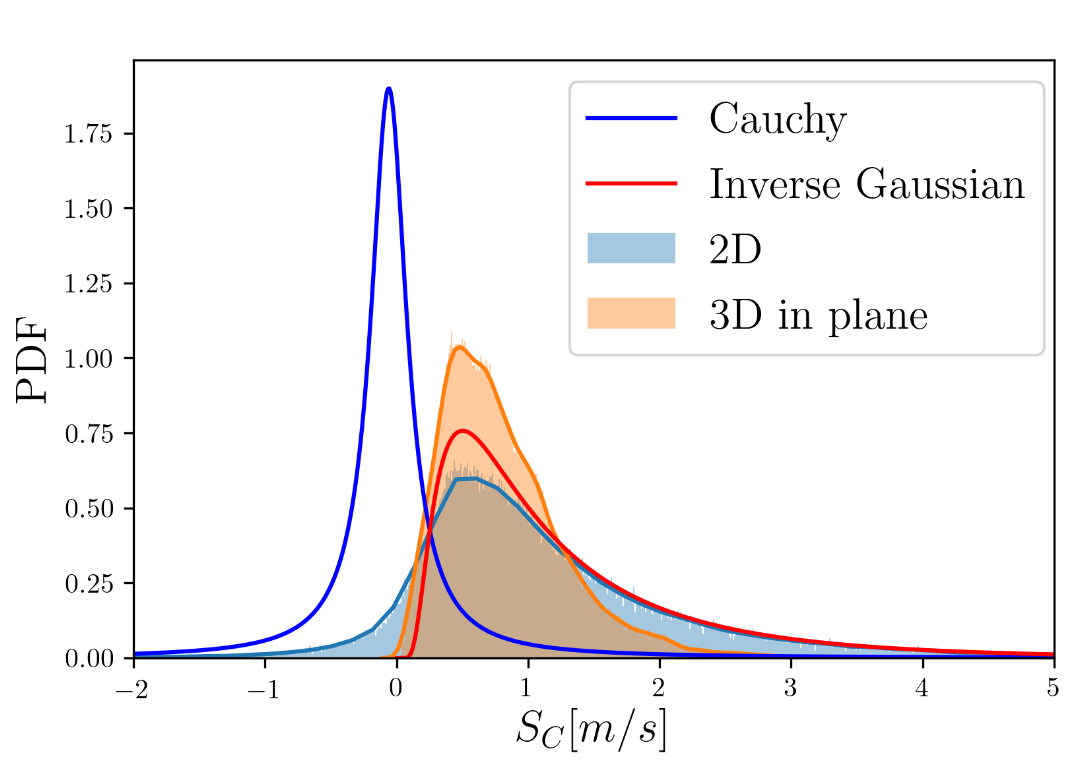
The 2D deconvoluted distribution results from this modeling approach are shown below. Comparing it to the 3D in plane consumption rates, we can see the it does a great job by estimating the lower values and does not include for the negative values; this is due to the use of the Inverse-Gaussian distribution. It does, however, over-estimates the larger positive values. In reality, these values would be attributed to other physical processes that can also be modeled and included in the mixture model.
